If you’re new to AI and want to have a deeper understanding and wondering where to begin, we’ve got you covered. We created this primer to learn the fundamental concepts of AI, from a single neuron in a network to transformers and LLMs. We’ve written it as a timeline so you learn not only the technical aspects of AI but also the way the field developed over the last 70 years.

AI is a field filled with lots of jargon like “hidden layers” and “neurons”. When you see the 🤓 emoji, this is where we go a layer deeper and explain the technical aspects behind the jargon. We’ve also included links to relevant papers and books in the field if you want to go even deeper.

This post is split into three parts, each taking about 15 minutes to read.

Part 1 - The Neural Network

1940s-1950s

You may be surprised to learn that the concept of abstracting the human brain into a computer dates back to the 1940s when neurophysiologist Warren McCulloch and logician Walter Pitts developed a mathematical model of an artificial neuron[1]. This work was then further developed by a psychologist named Frank Rosenblatt so that the artificial neuron could learn. He also worked on the first device that used the concept of the artificial neuron - the Mark I Perceptron in 1957[2]. Rosenblatt was able to successfully demonstrate that his artificial neuron could perform binary classification i.e. the ability to classify the elements of a given set into two groups (e.g. pictures of dogs vs pictures of cats.)

🤓 What is a perceptron?

Neurons are nerve cells in the brain that process and transmit chemical and electrical signals.

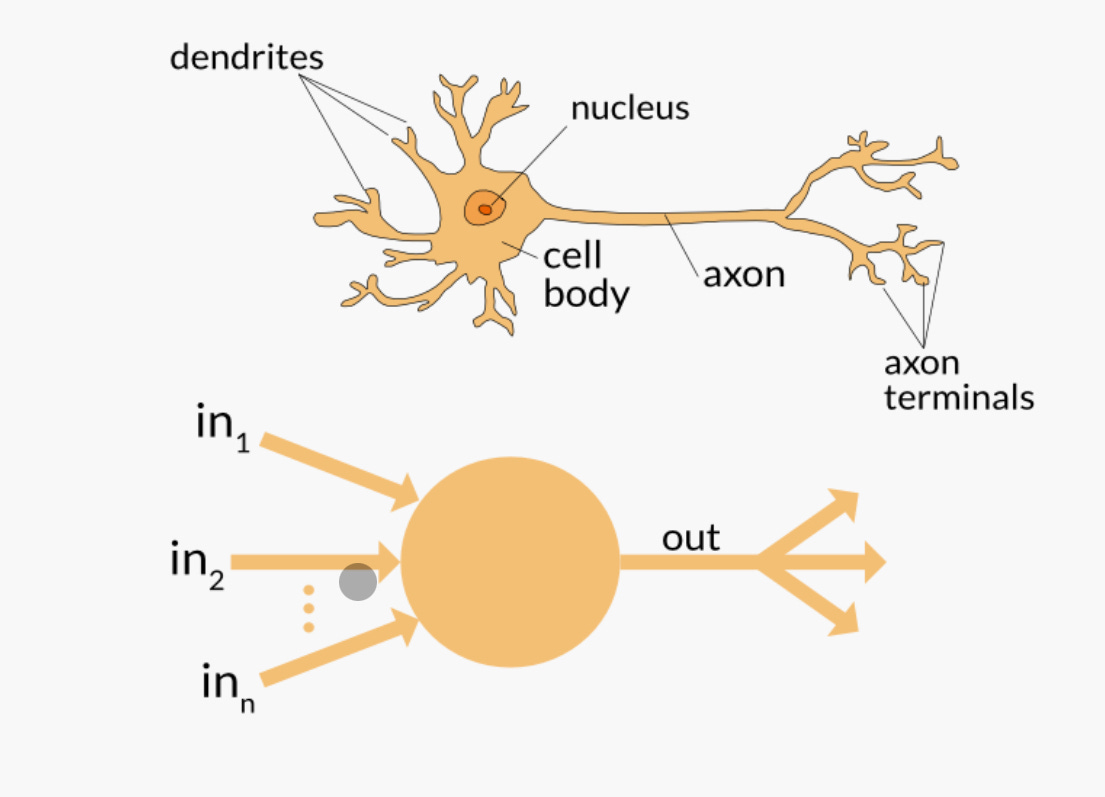
A perceptron is a type of artificial neuron, or "node," that is used in an artificial neural network. It is a simple model that is used to classify input data into one of two categories.

Here's how a perceptron works:

1. The perceptron receives input data in the form of numerical values called "features." The input data is multiplied by a set of weights, which are also numerical values used to adjust each feature's importance.
2. The weighted input values are then summed together, and the sum is passed through an activation function. The activation function determines whether the perceptron "fires" or activates based on the input.
3. If the perceptron activates, it outputs a "1." If it does not activate, it outputs a "0."
4. The perceptron's output is used to classify the input data into one of two categories. For example, if the perceptron outputs a "1," the input data might be classified as belonging to one category. If it outputs a "0," the input data might be classified as belonging to a different category.

Another way to think about a perceptron is a mathematical function with multiple weights w1, w2, w3… that multiply the input signals x1, x2, x3… and then are summed together.

If the sum is greater than some activation threshold θ, then the neuron activates, and the output is 1; otherwise, it is 0. We can represent this as the function f(z):

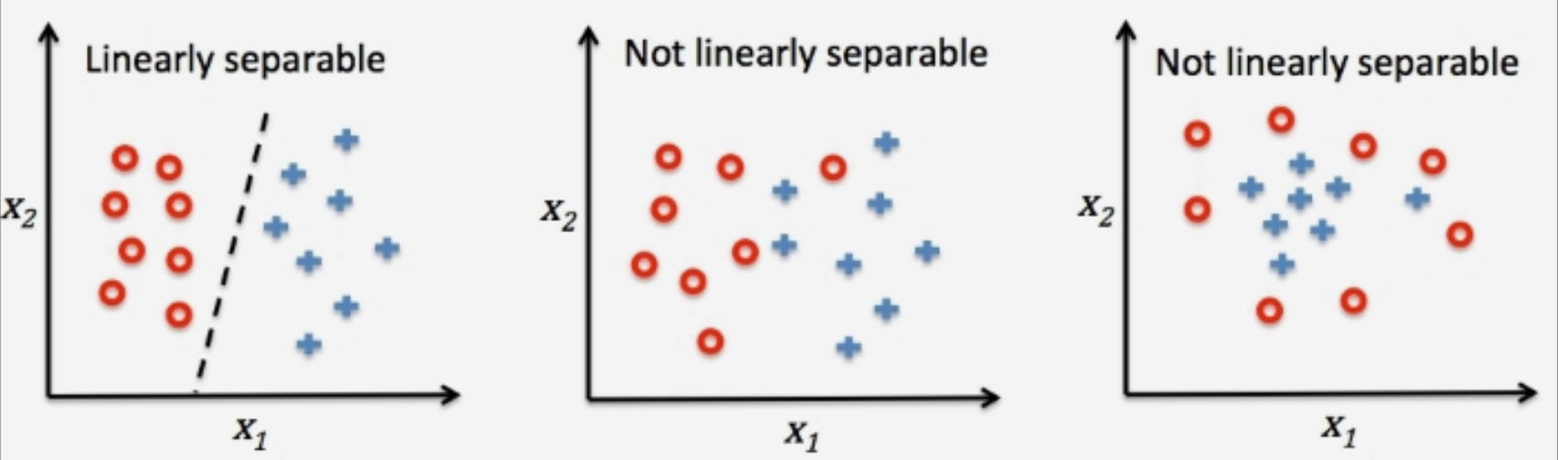
Using this function, we can now train a neuron to classify inputs into a binary set when they are linearly separable (i.e., you can draw a line between the two groups of inputs). We do this by changing the weights up and down until the neuron only fires when the input matches the expected output.

1960s

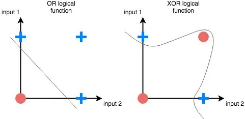
Marvin Minsky, an MIT professor, and Seymour Papert, a mathematician, published a book called Peceptrons[3] about Rosenblatt’s machine. The book showed that Rosenblatt’s perceptron was limited in its capabilities, like any other single-layer perceptron. Crucially, they showed that it can’t learn the simple logical function XOR, because it is non-linearly separable.

🤓 What does it mean to be linearly separable?

Data is linearly separable when the data points within that data can be separated into two classes using a straight line. For example, if we have a dataset of two classes, "dogs" and "cats," and the data points for "dogs" have a feature A = big ears and feature B = long tail, whereas data points for "cats" have feature A = small ears and feature B = short tail, it will be possible to draw a line in a 2D space to separate these two classes with all the "dogs" points on one side of the line and all the "cats" points on the other side.

As we’ll find out soon, the fact that single layer perceptrons can only separate data that is linearly separable end up being a huge limitation to its application.

1960s continued…

At the same time, in 1962, Arthur Samuel, a researcher at IBM, published an essay, “Artificial Intelligence: A Frontier of Automation,”[4] in which he defined a different way to get computers to complete tasks: Machine Learning.

🤓 What is Machine Learning?

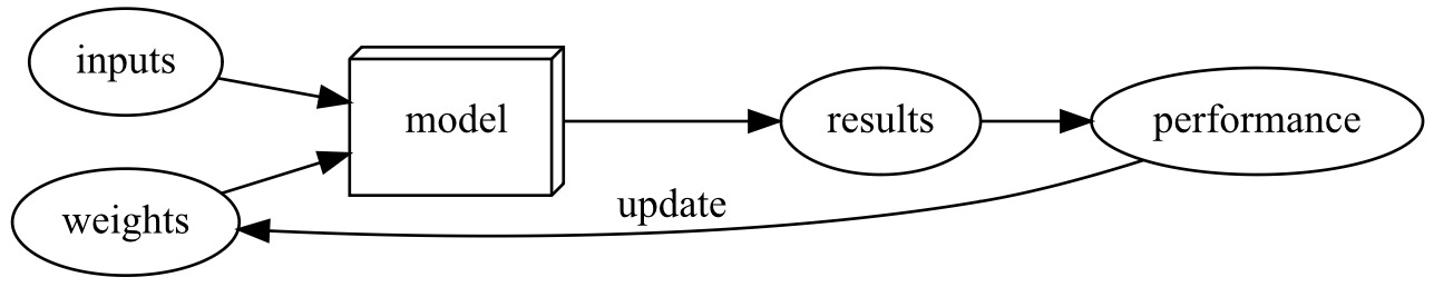
Unlike regular programming, Machine Learning does not take the approach of spelling out each step-by-step instruction to achieve a certain task. Instead, Machine Learning takes a set of input values and assigns some weights to those inputs that define how the input is processed in order to produce a specific result. This key difference changes the process from a program to a model. A model is a special type of program that can do many different things depending on the weights assigned to it.

But wait, isn’t that just a different type of program, like a recipe for cooking?

Not quite. The other big difference is that, unlike a recipe where ingredients' " weights " are constant, in Machine Learning, the weights are not constant. In fact, they themselves are variables that can change the way the inputs are processed depending on their assignment.

So how do we set the correct weights to get the best result?

In order to know if the weights are assigned to maximize performance, we need a way to automatically test the effectiveness of any weight assignment. We can do this by providing input data i.e., pictures of cats and dogs, and seeing if the resulting predictions are accurate or not.

OK, but what if the weight assignments are wrong and the results aren’t very good?

There’s a mechanism for automatically altering these weights to maximize the model's performance to achieve the best results called training the model.

Putting this all together, we have a process by which we assign weights to a model automatically and then alter these weights automatically, constantly testing the model’s result to maximize the performance. This combined process is what we call Machine Learning.

1970s

Advancements in the field of neural networks almost grind to a halt. Academics aren’t convinced of the usefulness of neural networks because of Minksy and Papert’s findings on the limitations of single layer perceptrons. Unfortunately they don’t recognize another crucial finding that Minksy and Papert also had in the same book: Multiple layers of perceptrons can represent more complex functions and data. The limited computational power of computers at the time also makes it difficult to train larger and more complex neural networks.

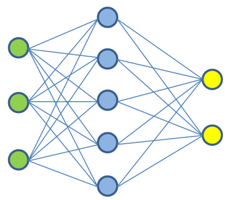
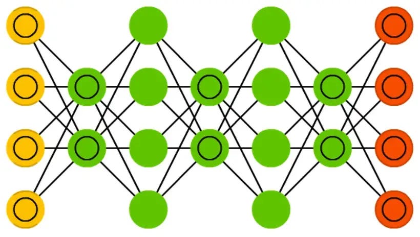
🤓 What is a neural network?

A neural network is a type of machine-learning model that is inspired by the structure and function of the human brain. It is composed of a large number of interconnected "neurons" (e.g., perceptrons) that are organized into layers. These layers process and pass information through the network in a way that allows it to learn and make predictions or decisions.

How does it actually work?

At a basic level, a neural network takes in inputs, performs computations on them, and produces outputs. The inputs are usually in the form of numerical values and are passed through the network, where the interconnected neurons process them. Each neuron performs simple mathematical computations on the inputs it receives and sends the result to other neurons in the next layer. In this way, the input data is transformed and distilled as it flows through the network, and eventually, an output is produced.

But not all data comes in the form of numerical values, for example, pictures?

Data is often preprocessed and transformed into numerical values before it is input into the network. This process is known as feature extraction or feature engineering.

For example, when working with image data, the raw pixel values of the image must be transformed into numerical values that the neural network can process. One way to do this is by normalizing the pixel values to a specific range, such as between 0 and 1, so that the network can more easily learn from the data. Another way is to extract features from the image, such as edges, corners, or color histograms, which can be represented as numerical values.

What about text data?

When working with text data, the text is typically tokenized and encoded as numerical values. Tokenization involves breaking the text into individual words or phrases, and encoding converts each word or phrase into a numerical value. This is often done using a technique called one-hot encoding, where a unique number is assigned to each unique word or phrase.

How do these neural networks learn things?

A neural network can learn by adjusting the strengths of the connections between the neurons, known as "weights," to minimize the difference between the output produced by the network and the desired output. This is done through a training process by providing the neural network with labeled data, allowing it to learn the mapping between inputs and outputs.

What are these neural networks used for?

Neural networks can be used for a wide range of applications, such as image recognition, natural language processing, speech recognition, and many others. They are particularly useful for tasks that involve large amounts of data and complex patterns, such as image and speech recognition.

1970s continued…

In 1974 however, Paul Werbos, who was studying for a Ph.D. at Harvard, invented an algorithm that was ignored for decades but today is an important foundational tool in the field of machine learning and neural networks: Backpropogation[5]. In his thesis, Werbos described the backpropagation algorithm and demonstrated its ability to train artificial neural networks to perform tasks such as function approximation and time series prediction. The backpropagation algorithm was later expanded upon and developed by other researchers and has become a fundamental tool in the field of machine learning.

🤓 What is backpropagation?

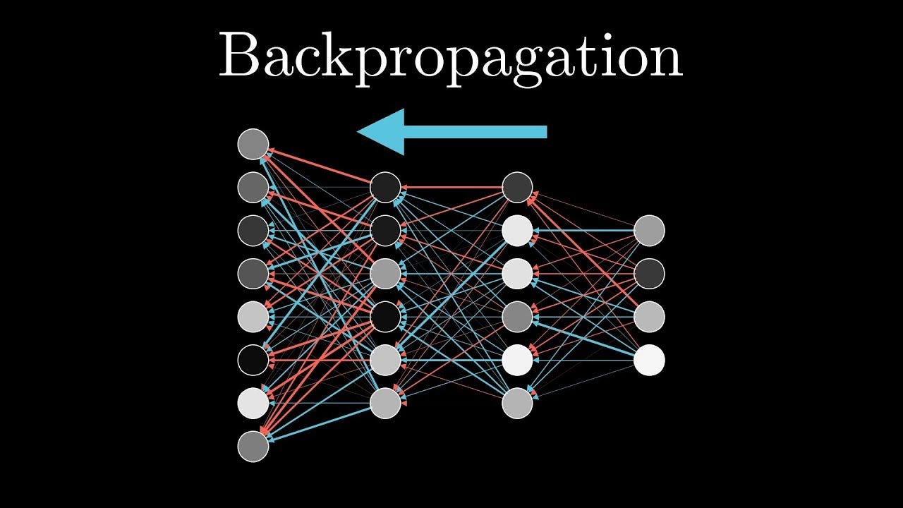
Backpropagation is a training algorithm for artificial neural networks that is used to calculate the error gradient of a network and adjust its weights of the network to minimize the error. The error gradient is a measure for each weight of how changing that weight will affect the loss of the model. Loss is just a function that measures the performance of a model i.e. how good it is getting the desired result. An ideal loss function returns a value that is a small loss when the model is performing well and a large loss when the model is performing poorly.

What’s a good example of a loss function?

One of the most common loss functions used in backpropagation is the mean squared error (MSE) loss function. MSE measures the average squared difference between the predicted output and the true output. The MSE loss function is often used in regression tasks, where the output is a continuous value.

How is a loss function used in backpropagation?

Here's how backpropagation works:

1. The neural network is presented with an input and makes a prediction. e.g., an image of a cat.
2. The prediction is compared to the true output, and the error is calculated. In this case we know the image is a cat, and we compare that to the prediction the model makes on how likely it is to be a cat.
3. The error is propagated backward through the network, and the weights of the network are adjusted to minimize the error. This is done by using an optimization algorithm, such as gradient descent, which adjusts the weights of the network in a way that reduces the error.
4. This process is repeated for many input-output pairs, and the weights of the network are continually adjusted to minimize the error.
5. The process is stopped when the error is below a certain threshold or when the weights of the network have converged to a stable solution.

Wait, what is gradient descent?!

Gradient descent is an optimization algorithm used to find a model's optimal set of parameters. Machine learning models often have many parameters that need to be set for the model to work properly. The goal of training a machine learning model is to find the values for these parameters that result in the best performance on the task at hand.

Gradient descent is an iterative algorithm that starts with an initial set of parameters and then iteratively improves them by moving in the direction of the negative gradient of the loss function. The gradient is a vector that points in the direction of the greatest increase in the loss function. By moving in the opposite direction of the gradient, the algorithm can find the set of parameters that minimizes the loss function.

The gradient descent process can be visualized as a ball rolling down a hill. The ball starts at the top of the hill and then rolls downhill, following the steepest descent until it reaches the bottom. The minimum of the loss function is represented by the bottom of the hill, and the ball's path down the hill represents the path taken by the algorithm to find the minimum.

If you want to go deeper into exactly how backpropagation and gradient descent works, check out this great Youtube video by Andrej Kaparthy (Tesla, Open AI):

Part 2 - Hidden Layers

We ended Part 1 at the close of the 1970s in the AI winter. Research has slowed down because of the limits of single-layer neural networks and computers not yet being powerful enough to train large networks.

Let’s pick things up in the 1980s…

1980s

As we learned in Part 1, single-layer neural networks are limited to only being able to learn linearly separable data, which means they can’t learn simple mathematical functions like XOR. In theory, adding just one additional layer to a single-layer network allows it to approximate any mathematical function. In practice, however, two-layer networks are too big and too slow to be useful.

Two-layer neural networks have many parameters which need to be adjusted during the training process. This requires a lot of computational resources, making the training process very slow, especially when working with large datasets. Two-layer neural networks are also limited to learning complex patterns and features from data. Because they only have two layers (input and output layer), they cannot extract high-level features that can be used to represent data beyond those directly represented in the input layer. This makes it difficult to learn complex relationships and patterns.

A great example of the limitations of a two-layer network is the task of image recognition. A two-layer neural network would only have an input layer that receives the raw image data and an output layer that produces the final prediction or decision. The lack of additional layers between the input and output layers limits the capacity of the network to extract high-level features such as edges, textures, and shapes from the image data.

In order to create neural networks that are more capable of learning, researchers would need to go beyond two layers. These multi-layer neural networks are called Deep Neural Networks (DNNs).

🤓 What is a Deep Neural Network?

A deep neural network (DNN) has many layers, typically composed of an input layer, multiple hidden layers, and an output layer. Each layer contains a set of interconnected "neurons" that perform computations on the input data and pass the results to the next layer. The neurons in a deep neural network are connected by weights which can be learned through training. The training goal is to adjust these weights so that the DNN produces the desired output for a given input.

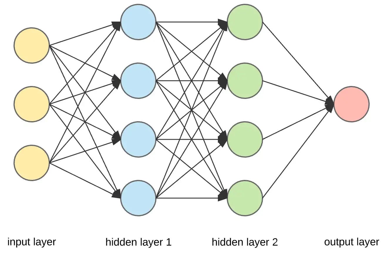
What are hidden layers?

The input layer takes in the input data, which is then processed by the hidden layers. The hidden layers are called "hidden" because their internal workings are not directly observable and are not part of the network's input or output. These layers use a set of weights and biases to transform the input data, passing it through multiple non-linear processing stages known as activation functions. The output of the last hidden layer is then passed on to the output layer, which produces the network's final output.

The purpose of the hidden layers is to extract and abstract features from the input data and pass them on to the next layer. The more hidden layers a DNN has, the more complex patterns it can learn and represent. The number of hidden layers and the number of neurons in each hidden layer is a parameter of the network called its architecture and can be adjusted during the training process to optimize the network's performance.

To simplify, think of a DNN as a function that can map input data to output data by passing through the layers. Each layer adapts the function to better fit the input-output pairs that it sees during the training phase, with the final output being the output of the last layer.

For example, let's say that the DNN is trained on a dataset of images of handwritten digits. During the training process, the DNN would learn the statistical patterns and relationships between the pixel values of the images and the labels indicating which digit the image represents.

Once the DNN is trained, it can be used to classify new images of handwritten digits. To classify a new image, the DNN would take the image's pixel values as input and pass them through the layers of the network, using the patterns and relationships it learned during training to classify the image as a specific digit.

1980s continued…

In 1986, a pivotal book was published: Parallel Distributed Processing (PDP) by David Rumelhart, James McClelland, and the PDP Research Group ^[6]. In the book, David Rumelhart and James L. McClelland explore using artificial neural networks for computational modeling. The PDP series includes several influential papers on developing neural networks and their applications.

One of the main contributions of the PDP series was the use of Paul Werbos’ backpropagation algorithm for training neural networks. The PDP series also introduced the concept of distributed representation, which is the idea that the meaning of a concept can be represented by the pattern of activity across multiple neurons in the network. This idea is important because it allows neural networks to learn more complex relationships between the input and output data and to generalize better to new data.

1990s

In the 1990s, the term "deep learning" is coined by Igor Aizenberg and colleagues to describe multi-layered neural networks. However, the biggest breakthrough of the decade was when Yann LeCun, Yoshua Bengio, and Geoffrey Hinton demonstrated the first successful application of deep learning in their work on handwritten digit recognition using a convolutional neural network (CNN)^[7].

LeCun’s, Bengio, and Hilton’s work is seminal because it demonstrates the effectiveness of deep learning for real-world applications. Prior to this work, there had been limited success in using neural networks for practical tasks, and many researchers were skeptical of their potential. However, the results of this work show that deep learning can be used to achieve high accuracy on a challenging real-world task, paving the way for further research and development in the field.

Here’s LeCun demo-ing his CNN, LeNet 1 in 1993:

🤓 What is a Convolutional Neural Network?

A convolutional neural network (CNN) is a type of deep neural network that is commonly used in image and video recognition tasks. It is designed to automatically and adaptively learn spatial hierarchies of features from input data, making it particularly well-suited for image analysis.

A CNN consists of multiple layers of interconnected neurons, which process and analyze the input data. The layers of a CNN are organized to learn increasingly complex features of the input data as the data passes through the network.

Why is it “convolutional”?

One key feature of CNNs is the use of "convolutional" layers, which are designed to automatically learn and extract features from the input data. These layers apply a set of filters to the input data and use the resulting output to detect patterns or features in the data. This process is repeated multiple times, allowing the CNN to learn increasingly complex features of the input data as it passes through the network.

Here’s a great video by Google that visualizes how a CNN works:

1990s continued…

In 1995, Jurgen Schmidhuber and his student Sepp Hochreiter publish a paper on the concept of "long short-term memory" (LSTM) units ^[8]

, which are a type of Recurrent Neural Network (RNN) that are able to capture long-term dependencies in time series data.

Traditional RNNs have difficulty in capturing long-term dependencies (e.g. one word after another in a sequence of text), which can limit their effectiveness for certain tasks. To address this issue, Schmidhuber and Hochreiter introduce the concept of LSTM units, which are able to "remember" information for long periods of time and use it to make predictions or decisions later. They demonstrate the effectiveness of LSTM units for a number of tasks, including language modeling and polyphonic music modeling, and show that they outperformed traditional RNNs in these tasks.

LSTMs go on to have a significant impact on the development of deep learning models for tasks such as language modeling, machine translation, and speech recognition.

🤓 What is a Recurrent Neural Network?

A recurrent neural network (RNN) is a type of artificial neural network that is designed to process sequential data, such as text or time series data. It is called "recurrent" because it uses sequential information, passing the output from one step of the processing back into the network as input for the next step.

How does an RNN work?

In a recurrent neural network (RNN), the neurons are connected in a directed cycle, meaning that the output from one step in the processing is passed as input to the next step in the cycle. This allows information to be passed from one step to the next and for the network to use information from the past to inform its current and future processing. For example, predicting where an object is going based on its passed co-ordinates or predicting the next word in a text based on previous words for auto-completion.

For example, in a language modeling task, an RNN might take a sequence of words as input and use the output from processing the previous word to inform its processing of the current word. This allows the RNN to capture the context and dependencies between words, which is important for understanding the meaning of the text.

What about LSTMs? How do they fit in?

A long short-term memory (LSTM) unit is a type of recurrent neural network (RNN) that is able to capture long-term dependencies in time series data. It is called "long short-term memory" because it is able to remember information for long periods of time and use it to make predictions or decisions later. For example, storing a whole sentence in a text to predict the next word vs just storing the last word.

What are RNNs useful for?

RNNs are particularly well-suited for tasks such as language modeling, machine translation, and speech recognition, where the order and context of the input data is important. They have also been applied to a wide range of other tasks, including image and video analysis, music generation, and protein folding prediction.

Here’s a great article that explains RNNs in more detail: Introducing Recurrent Neural Networks.

We end Part 2 with deep learning making steady progress thanks to the dedicated work of a small group of researchers, including Yann LeCun, Yoshua Bengio, and Geoffrey Hinton. During this period, many of their academic papers were rejected by journals and conferences because of their use of neural networks, despite dramatically outperforming any previous approaches.

In 2018, LeCun, Bengio, and Hinton were awarded the Turing Award, the highest honor in Computer Science, for their dedication and persistence in developing neural networks despite skepticism from the academic world.

‍

Part 3 - The AI Spring

We ended Part 2 at the turn of the century with a small group of dedicated researchers pushing forward the field of neural networks, despite the skepticism of the wider academic community. Meanwhile, limitations in computing power at the time made it harder to train larger models to solve more complex problems.

So how did we get from the AI winter of the 70s, 80s, and 90s to the exponential advancements we’re experiencing today? Let’s pick things up in the 2000s, where we rejoin Geoffrey Hinton and his team…

2000s: Deep Learning Accelerates

In the 2000s, Hinton and his team continue to make major advancements in deep learning, building on the foundation laid in the 1990s. They develop new training algorithms that improve the effectiveness of deep learning models, particularly Deep Neural Networks (DNNs). Their most notable contributions include "pre-training" and "fine-tuning," which they first successfully use in creating Deep Belief Networks (DBNs) in 2006 ^[9].

Hinton and his team propose a way to train neural networks by starting with simpler networks first and then building on top of them. This "pre-training" method helps the deeper networks learn more effectively. After pre-training, the team fine-tuned the network by adjusting it using a method called "supervised learning." This helped the network improve its performance even further. Deep Belief Networks were among the first successful examples of deep learning architectures that used pre-training, fine-tuning and unsupervised learning.

🤓 What is a Deep Belief Network?

Deep Belief Networks (DBNs) are a type of neural network trained using a special technique called unsupervised learning. This means the network is not given specific answers or expected outputs to learn from. Instead, the goal of a DBN is to find patterns and structures in the data on its own.

One example of how this works is in image recognition. Imagine we have a dataset of images of handwritten digits, and we want to train a DBN to recognize these digits. The visible layer of the DBN would represent the pixels of the images, and the hidden units would be used to identify the underlying structure of the images. For example, the hidden units might learn to recognize edges, corners, and other simple shapes in the images. These simple shapes can then be combined to form more complex ones like digits.

However, DBNs differ from Deep Neutral Networks (DNNs) and Convolutional Neural Networks (CNNs) covered in Part 2. DNNs use hidden layers to extract abstract and higher-level features from the input data, while CNNs use filters to identify specific image features. On the other hand, DBNs are unsupervised and learn the actual structure of the image that can later be combined to generate new images.

A key component of DBNs is the use of Restricted Boltzmann Machines (RBMs). RBMs are a type of neural network comprising two layers: a visible layer and a hidden layer. The visible layer represents the input data, and the hidden layer is used to learn a compressed representation of the input data. RBMs are probabilistic generative models, meaning they can learn the probability distribution of the input data and generate new samples that are similar to the training data.

In a DBN, multiple RBMs are stacked on top of one another. Each RBM learns a more abstract and higher-level representation of the data as it progresses through the network. This is similar to how a puzzle has many pieces that need to be put together to form a complete picture. The idea is that by stacking multiple RBMs, the DBN can learn a more detailed and accurate representation of the input data.

Once the DBN has been pre-trained using these stacked RBMs, it can then be fine-tuned using a labeled dataset and supervised learning techniques, such as backpropagation, to improve its performance on a specific task. This is similar to how a detective would use clues from a crime scene to make an arrest.

Overall, Deep Believe Networks have been used in various applications, such as image and speech recognition, and have played a significant role in the advancement of deep learning.

2000s continued: Off to the races!

As the decade proceeds, advancements in deep neural networks and the availability of large-scale datasets like Fei-Fei Li’s ImageNet ^[10]

and pre-trained models make deep learning much more approachable. Researchers no longer need expensive, time-consuming data collection and annotation to train, effective deep-learning models. This leads to an era of competitive research, with teams from around the world seeing who trains the most accurate models.

One of these competitions is the Netflix Prize. The aim of the competition is to use machine learning to beat Netflix's own recommendation software's accuracy in predicting a user's rating for a film, given their ratings for previous films by at least 10%. The prize was won in 2009 by BellKor's Pragmatic Chaos, a team whose members include employees of AT&T and Yahoo.

At the same time, another development comes along that literally accelerates the field of deep learning: The use of Graphics Processing Units (GPUs) in deep learning makes it possible to train large neural networks much more quickly than when using traditional processors on a computer.

🤓 Why do GPUs accelerate deep learning?

A GPU, or Graphics Processing Unit, is a type of computer chip that is specifically designed to process large amounts of data quickly and efficiently. They were originally created for use in video game graphics, but scientists and researchers soon realized that they could be used to accelerate many other types of computations, including those used in deep learning models.

Deep learning models, such as neural networks, typically involve a lot of complex mathematical calculations and require a lot of data to be processed at the same time. Training these models can take a long time on a regular computer, even with a fast processor.

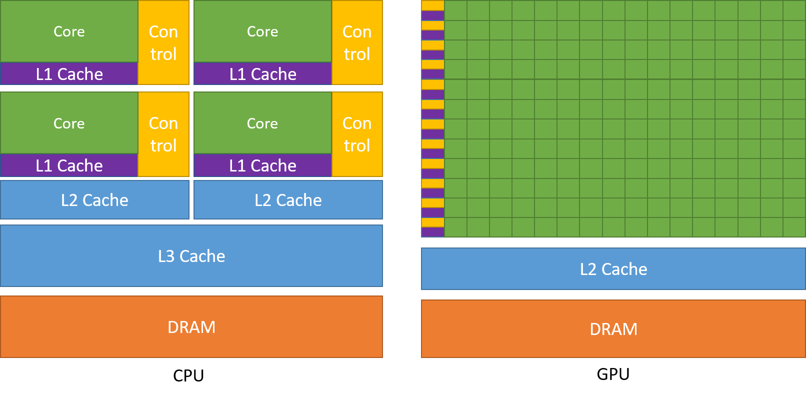
A CPU (Central Processing Unit) is divided into multiple cores so that they can take on multiple tasks simultaneously (e.g., browsing the internet while listening to Spotify). A GPU, on the other hand has hundreds and thousands of cores, which are dedicated to completing simple computations that are performed more frequently and independently of each other i.e. in parallel.

Training neural networks is an ideal task for GPUs. Calculating weights and activation functions of each layer and backpropagation can all be computed in parallel. A GPU is designed to handle these types of calculations much more efficiently. It can perform many calculations in parallel, which means it can work on many pieces of data at the same time. This allows deep learning models to be trained much faster on a GPU than on a regular computer.

As deep learning has progressed, it needs to have vast amounts of data to be fed and training on these data set takes a long time on a single CPU. With a single GPU, the time to train these models is significantly reduced, and with multiple GPUs working together in parallel, it's even faster.

2010s: “Hey Google…”

Thanks to the progress of the previous decade, the 2010s see exponential advancement in deep learning, with Apple, Google and Amazon all making major investments in the space ushering in the dawn of consumer-friendly AI. From automatically organizing your photos to helping you turn on the lights in your home and playing your favorite songs at the command of your voice, AI enters the mainstream and consumers lives.

The decade began with a seminal paper in 2012 by Geoffrey Hinton, Alex Krizhevsky and Ilya Sutskever that showed a massive leap in image recognition accuracy using deep neural networks ^[11]. Hinton and his colleagues developed AlexNet, a convolutional neural network that won several competitions.

In 2013 the film “Her” is released. A science fiction drama starring Scarlett Johansson as Samantha, an AI operating system who its user Theodore falls in love with. Samantha is portrayed as a highly intelligent and empathetic AI that is able to form a deep connection with Theodore. The film provides a very tangible sense of what the near future might look like with AI as part of our lives. At the same time, it also highlights the limitations of “AI Assistants” like Google Home, Siri, and Echo, which are far more limited in their ability.

🤓 How do voice assistants like Google Home, Siri and Echo work?

Remember from Part 2 how recurrent neural networks (RNNs) with long short-term memory are able to process longer sequences of input? That’s perfect for the use case of speech recognition in voice assistants, where a user makes a request with multiple words in a sequence.

RNNs work by using a feedback loop, where the output of a previous step is fed back into the network as input for the next step. This allows the network to "remember" what it has heard in the past and use that information to understand the current input better.

LSTMs are a type of RNN that are particularly well-suited for handling speech data. They use a special structure called a memory cell, which can retain information for long periods of time and selectively choose which information to discard and which to keep. This allows LSTMs to effectively filter out irrelevant information, such as background noise, and focus on the important parts of the speech input, which is critical in the use case of Voice Assistants.

RNNs and LSTMs form the backbone of AI voice assistants, allowing them to understand and respond to human speech in real time. As more data is fed into these networks, they continue to learn and improve, making them even better at understanding and responding to human speech.

It is worth mentioning that these models are trained on a massive amount of data; this allows them to generalize well and adapt to different accents, dialects, and speaking styles. It also allows them to understand and respond to new words and phrases and recognize and respond to specific speakers.

But voice assistants aren’t just tasked with recognizing speech. They also respond to a user’s commands by synthesizing human-like speech too. For example, if you ask Google Home, “What’s the weather like today?” It will respond with an answer describing the current weather conditions and forecast for the rest of the day. This is where deep neural networks (DNNs) and convolutional neural networks (CNNs) come into play.

In speech synthesis, deep neural networks (DNNs) and convolutional neural networks (CNNs) model the complex relationships between audio signals and human speech. These models are trained on large amounts of speech data to recognize patterns associated with different speech sounds, such as phonemes and words. They are then used to generate new speech from text by predicting the most likely sequence of speech sounds.

It’s worth noting, however, that voice assistant are limited in their ability because they are based on a set of predefined rules and commands. They are not truly intelligent because they do not have the ability to learn and adapt like a human would. They rely on a set of programmed responses and cannot understand the context or make decisions based on new information.

2010s continued: The race to general intelligence begins

In the 2010s, startups like OpenAI and Deepmind (acquired by Google in 2015 for over $400M) were funded with the explicit goal of achieving Artificial General Intelligence (AGI). AGI is a type of artificial intelligence designed to possess a broad range of cognitive abilities similar to those of a human being. This includes the ability to understand complex concepts, reason, plan, solve problems, and learn from experience similar to our idea of AI from sci-fi movies like “Her”. This new injection of capital into AI research from startups and big tech companies spurs an exponential increase in advancements in the field.

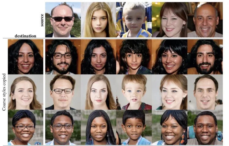
One of these new developments is generative models. These models are designed to generate new output data rather than classify or recognize input data. One of the most popular early generative models is the Generative Adversarial Network (GAN) which was introduced by Ian Goodfellow in 2014 ^[12]. The main advantage of GANs is the ability to generate new data that is similar to the training data, allowing them to be used for tasks such as image synthesis, image-to-image translation, and other generative tasks.

🤓 What is a Generative Adversarial Network (GAN)?

Generative Adversarial Networks (GANs) are a class of generative models that use a technique called adversarial training, where two neural networks, a generator, and a discriminator, are trained together.

The generator network learns to generate new data samples that are similar to the training data. It takes in a random noise as input, producing a new data sample similar to the training data. The generator is typically a neural network with an architecture designed to produce new data samples, such as a decoder network.

The discriminator network, on the other hand, takes in both real data samples from the training set and fake data samples generated by the generator. It is trained to distinguish between the real data samples and the fake data samples generated by the generator. The discriminator is also typically a neural network but with an architecture designed to distinguish between real and fake data samples.

The training process of a GAN is an adversarial process where the generator and discriminator are trained simultaneously and in opposition. The generator is trained to produce data samples that can fool the discriminator into thinking they are real, while the discriminator is trained to correctly identify the real data samples from the fake ones generated by the generator.

At the beginning of the training, the generator produces poor-quality samples, the discriminator easily recognizes them as fake, and thus the generator is updated to improve its performance. As the training progresses, the generator improves and generates better-quality samples, making it harder for the discriminator to distinguish between real and fake data. The discriminator also improves by training on both real and fake samples. The training continues until the generator produces samples that fool the discriminator.

This process is called adversarial training; the generator and discriminator are competing with each other, and the generator is trying to produce realistic samples that the discriminator would not be able to tell apart from the real ones. This leads to the generator learning to produce samples that are similar to real ones.

2010s continued: Transformers - More than meets the eye?

Arguably one of the most revolutionary breakthroughs in deep learning in the 2010s is the invention of the Transformer architecture in 2017 by Google researchers in the famously titled paper “Attention is All You Need” ^[13]. In the paper, Google’s researchers propose “a new simple network architecture, the Transformer, based solely on attention mechanisms, dispensing with recurrence and convolutions entirely.”

The advent of the Transformer architecture has played a significant role in developing large-scale language models (LLMs) such as OpenAI’s GPT-3, which powers ChatGTP. These Large-scale language models are essentially transformer-based architectures that are trained on large amounts of text data, and have billions of parameters, which allows them to understand the input more effectively, generate more coherent and human-like text, and generalize better on unseen examples.

Before the transformer architecture, Recurrent Neural Networks (RNNs) were the most commonly used architecture for language modeling tasks. However, RNNs are not well-suited for processing long text sequences and have difficulty learning long-term dependencies in the input.

🤓 What is the Transformer architecture?

Remember from earlier that recurrent neural networks and convolutional neural networks store a fixed length part of their input in memory in hidden layers to better predict the output. The challenge with this approach is that it requires the model to process its input serially, for example, processing a paragraph of text one word at a time. This process cannot be parallelized when training which creates challenges due to limitations in memory. It also limits how far back a model can learn about the text it is trained on for any word in the text, referred to as “lookback.”

The transformer architecture is based on the idea of allowing the model to look at the whole sequence of input rather than a fixed-length part of the input like recurrent neural networks with long short-term memory do. Then the model focuses on certain parts of that input that are relevant to each word. It achieves this through a mechanism called self-attention, which you can liken to being able to look up different words in a dictionary.

Attention was first introduced in 2015 in the context of language translation from English to French. In the paper, the authors gave the example of translating the following English sentence:

“The agreement on the European Economic Area was signed in August 1992.”

Into the French equivalent:

“L’accord sur la zone économique européenne a été signé en août 1992.”

Trying to translate this sentence by going through each English word individually wouldn’t work for many reasons: some French words are flipped, and the French language has gendered words.

Attention is a mechanism that allows the model to focus on every single word in the French input when generating the English output and pay more attention to specific words.

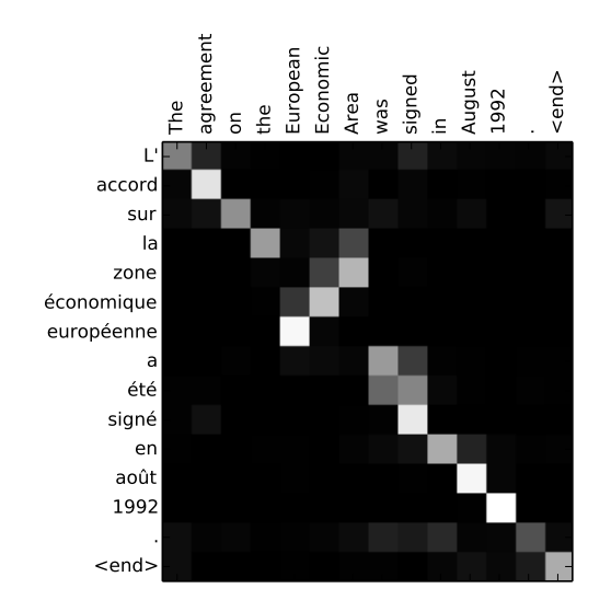
The model learns which words it should “attend” to from training data by processing thousands of French and English sentences.

Unlike regular attention, self-attention doesn’t look at the attention of specific words for a given input and output, as this is limited to translations. Instead, it looks at the attention to give different words in the input for each word in the input itself. In order words, self-attention allows a neural network to understand a word in the context of words around it. This is important in NLP tasks such as language understanding, where the meaning of a word depends on the context and its relationship with other words in the sentence.

The transformer architecture also introduced the concept of multi-head attention, which enables the model to attend to multiple parts of the input simultaneously, improving the model's performance by allowing parallelization.

Additionally, the transformer architecture introduced the concept of position encoding, which allows the model to understand the order of the tokens in the input and make use of their relative position to understand the meaning of the input better.

2018: BERT - The first breakthrough Large Language Model

In 2018, Google researchers introduced BERT (Bidirectional Encoder Representations from Transformers), the first breakthrough large language model [14]. BERT uses the Transformer encoder architecture and is trained on a large corpus of text using two unsupervised prediction tasks: masked language modeling and next sentence prediction.

BERT's key innovation was pre-training the model on a large amount of text data before fine-tuning it for specific tasks. This allowed BERT to learn general-purpose representations of language that could then be adapted for various NLP tasks.

At the time of its release, BERT set new state-of-the-art results on a wide range of NLP tasks, including question answering, natural language inference and sentence similarity. This demonstrated the effectiveness of large pre-trained language models for improving the performance of NLP systems.

BERT used a Transformer-based model with 110 million parameters, which was considered large at the time. However, it pales in comparison to today's large language models like GPT-3 which have billions of parameters.

BERT's breakthrough success demonstrated the potential of large pre-trained language models and spurred a wave of follow-up research to develop even larger and more capable models. BERT laid the foundation for today's state-of-the-art large language models and generative AI systems.

🤓 How do large-scale language models like BERT and GTP work?

A large-scale language model (LLM) is a type of deep learning model that is trained on a large dataset of text (e.g. all of the internet). LLMs predict the next sequence of text as output based on the text that they are given as input. They are used for a wide variety of tasks, such as language translation, text summarization, and generating conversational text. Open AI’s GPT-3 (General Pre-trained Transformer 3) ^[15]

, the language model that powers Chat-GPT, is an example of a generative LLM that uses the Transformer architecture, enabling it to be trained on a massive text dataset of hundreds of gigabytes using 175 Billion parameters (weights assignments).

GPT-3’s size made it the largest language model at the time of its launch though it was later superseded by Google’s PaLM which boasts over 540 billion parameters. GPT-3s use of the Transformer architecture allows it ot understand and generate language in a way previous models could not. It also used unsupervised learning, to be trained without any specific task in mind. This allows it to be fine-tuned for a variety of different tasks, such as text completion, question answering, and language translation.

Once LLMs get to this size, they start exhibiting emergent behavior, unexpected and seemingly autonomous actions or decisions that the model makes due to its training on the vast amount of data it has been exposed to. This can be seen in GPT-3's ability to generate human-like text that is often difficult to distinguish from text written by a human. However, it is important to note that this behavior is not truly autonomous, as it is still determined by the patterns and connections present in the training data.

Additionally, GPT-3's may generate text that appears to have a bias or hold certain beliefs, which reflects the biases and beliefs present in the training data, highlighting the need for diverse and unbiased data when training such models. These large models are also prone to “hallucinations”, the term in AI for when a model makes up an answer in a way that appears to be factual but is not. For example, it may generate a citation to an academic paper that looks real but has the incorrect authors!

Present Day: The Generative AI Revolution

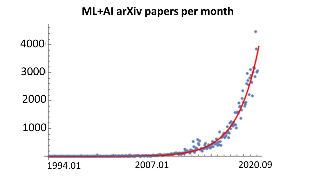
Fast forward to 2023 and thanks the over a 70 years of advancements in AI we're now starting to see AI dramatically change the way we live, work and play. From ChatGPT taking the world by storm just 6 months ago and already rumored to be generating $1B in revenue to robotaxis taking over the streets of San Francisco and AI-generated images taking over the internet, we're entering a golden age of AI. At the same time advances in AI seem to be exponentially increasing as well funded companies like Google and OpenAI compete to outdo each other with the capabilities of their large language models. The open-source community is also thriving thanks to communities like HuggingFace, open-source models like LLaMA and the wave of talented people that are now contributing to thousands of open source projects. And then of course there's the startup ecosystem where despite a broader downturn, billions of dollars of capital are now being invested in AI startups that are using AI to revolutionize many industries including marketing, sales, customer support, software engineering and even compliance and operations.

In reflecting on how we got here though, it’s important to realize and appreciate the tireless efforts of researchers and engineers who laid the foundations for the incredible progress seen in deep learning today. Even, a decade ago, there were doubts about the effectiveness of neural networks that persisted until companies like Google invested billions of dollars into advancing the field. Thanks to all these efforts, innovating in AI is now more approachable than it ever was before. It's entirely possible that the next big breakthrough could come even come from an AI startup. For example, at Parcha the work we're doing to build AI Agents to automate manual workflows is at the bleeding edge of Applied AI. We're tackling challenges like reducing hallucinations, getting agents to carry out complex operational tasks and even the process of creating AI Agents using generative AI.

If you are excited about contributing to what is likely to be the most impactful technology shift in our generation and possibly ever, we would like to hear from you. We're hiring experienced software engineers that are curious about AI with not prior experienced required. To learn more or check out our jobs page.

AI is going to change the world around us and we're just getting started!

Footnotes

[1] - McCulloch, W. S., & Pitts, W. (1943). A logical calculus of the ideas immanent in nervous activity. The bulletin of mathematical biophysics, 5(4), 115-133.

[2] - Rosenblatt, F. (1957). The perceptron, a perceiving and recognizing automaton Project Para. Cornell Aeronautical Laboratory.

[3] - Minsky, M. L., & Papert, S. A. (1969). Perceptrons: An introduction to computational geometry.

[4] - Samuel, A. L. (1962). Some studies in machine learning using the game of checkers. IBM Journal of research and development, 3(3), 210-229.

[5] - Werbos, P. J. (1974). Beyond regression: New tools for prediction and analysis in the behavioral sciences (Doctoral dissertation, Harvard University).

[6] - Rumelhart, D. E., McClelland, J. L., & Group, P. R. (1986). Parallel distributed processing (Vol. 1). Cambridge, MA: MIT press.

[7] - LeCun, Y., Bottou, L., Bengio, Y., & Haffner, P. (1998). Gradient-based learning applied to document recognition. Proceedings of the IEEE, 86(11), 2278-2324.

[8] - Hochreiter, S., & Schmidhuber, J. (1997). Long short-term memory. Neural computation, 9(8), 1735-1780.

[9] - Hinton, G. E., Osindero, S., & Teh, Y. W. (2006). A fast learning algorithm for deep belief nets. Neural computation, 18(7), 1527-1554.

[10] - Deng, J., Dong, W., Socher, R., Li, L. J., Li, K., & Fei-Fei, L. (2009, June). Imagenet: A large-scale hierarchical image database. In 2009 IEEE conference on computer vision and pattern recognition (pp. 248-255). Ieee.

[11] - Krizhevsky, A., Sutskever, I., & Hinton, G. E. (2012). Imagenet classification with deep convolutional neural networks. Advances in neural information processing systems, 25, 1097-1105.

[12] - Goodfellow, I., Pouget-Abadie, J., Mirza, M., Xu, B., Warde-Farley, D., Ozair, S., ... & Bengio, Y. (2014). Generative adversarial nets. Advances in neural information processing systems, 27.

[13] - Vaswani, A., Shazeer, N., Parmar, N., Uszkoreit, J., Jones, L., Gomez, A. N., ... & Polosukhin, I. (2017). Attention is all you need. Advances in neural information processing systems, 30.

[14] - Devlin, J., Chang, M. W., Lee, K., & Toutanova, K. (2018). Bert: Pre-training of deep bidirectional transformers for language understanding. arXiv preprint arXiv:1810.04805.

[15] Brown, T. B., Mann, B., Ryder, N., Subbiah, M., Kaplan, J., Dhariwal, P., ... & Amodei, D. (2020). Language models are few-shot learners. arXiv preprint arXiv:2005.14165.

‍